Investing With Training Wheels: How Buffer ETFs Can Help Mitigate Risk
Here's a look at how structured outcome ETFs can help limit volatility and drawdowns for investors with a lower risk profile.

Do you remember learning to ride a bike? Chances are, you started with training wheels. As adults, we might scoff at them now, but back then, they were invaluable—keeping you from falling down as often or as hard. Sure, they limited your speed and agility, but the trade-off for extra safety was worth it.
It turns out you can use a similar concept in investing to help reduce volatility and limit losses. While some people lean on high-quality bonds or low-beta stocks, another approach involves derivatives.
Unlike strategies reliant on correlations¹ holding steady, derivatives are grounded in math—designed to deliver structured outcomes regardless of broader market behavior.
If you’re a risk-conscious investor (and let’s be honest, in today’s uncertain markets, who isn’t?), buffer ETFs offer another way to protect your portfolio. Here’s how these specialized ETFs work and why they might be worth a look.
Why investors should care about risk
If you’d invested $10,000 in the S&P 500 from August 31, 1976, to December 11, 2024, the results on paper look spectacular: a 10.56% compound annual growth rate (CAGR)² turning that initial sum into a staggering $1,271,197.03³.
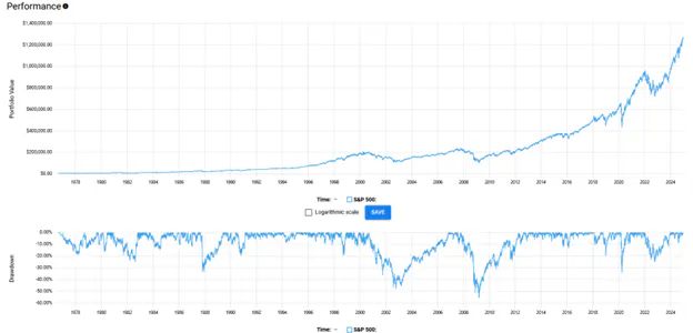
Source: testfolio.io as of December 13, 2024.
What’s the catch? It assumes one critical thing—that the hypothetical investor stayed the course, never panicked, and avoided trying to time the market. That’s far easier said than done, thanks to two significant sources of risk: volatility and drawdowns.
Volatility⁴, measured by standard deviation, reveals the typical ups and downs in the market. For this investment, the standard deviation sat at 17.54%. What does that mean? Historically, there has been instances where our hypothetical investor watched their portfolio swing dramatically in value, sometimes by tens of thousands of dollars in a single year. The more money you have, the more nerve-wracking these fluctuations can become.
Then there’s the maximum drawdown—the peak-to-trough drop during a crisis. In this case, the 2008 financial crisis saw our investor’s portfolio plummet 55.26%, shrinking from over $200,000 to just over $100,000 in a matter of months. Imagine watching half your portfolio evaporate, with no guarantee at the time it would ever recover.
Ask yourself this: even knowing in hindsight that things worked out, could you have stayed the course during such a catastrophic drawdown? If the answer is no, then perhaps limiting both the ups and downs of your investments might help you sleep better at night.
How buffer ETFs work
Buffer ETFs could therefore be a solution for reducing these emotional and financial roller coasters. To put it simply, these ETFs employ the financial equivalent of “training wheels” to limit the range of investment results over a time period – hence the name “structured outcome”.
Buffer ETFs aim to protect against market declines while allowing for participation in the upside, up to a pre-determined limit. Of course, this protection comes with a trade-off: giving up some of the upside potential in exchange for reduced downside risk.
But this can be particularly useful given the asymmetric nature of returns and losses—for instance, a 10% loss requires an 11.1% gain to break even, a 25% loss requires a 33.3% gain, and a 50% loss needs a whopping 100% recovery just to get back to square one⁵.
A buffer ETF is pegged to the price return of a reference asset, such as the S&P 500 index, and employs an options overlay to create the buffer. For example, BMO’s buffer ETFs offer a 15% buffer, meaning the ETF absorbs the first 15% of losses in the reference asset during a set time period.
If the market falls by 12%, the ETF absorbs the entire loss, leaving the investor unscathed. However, if the market declines by 20%, the investor will still experience a 5% loss beyond the buffer.
This protection doesn’t come for free. The cap, or maximum return you can achieve with the ETF, offsets the cost of the buffer. Essentially, options are sold to fund the protection, which limits the investor's participation in upside gains.
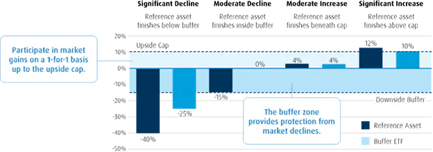
Source⁶: BMO Global Asset Management as of December 13, 2024.
Understanding the fine print
One important aspect to note is that buffer ETFs are tied to specific outcome periods which usually is one year. The start of the outcome period usually corresponds to a calendar month. For BMO’s buffer ETFs, these periods and their corresponding caps and buffers are as follows:
Data as of October 1, 2024. Starting cap and buffer is before fees, expenses, and taxes⁷.
Why is this important? The indicated cap and buffer only apply if you buy the buffer ETF on the start date of the target outcome period and hold it until the end. If you purchase the ETF in between these dates, some of the cap and buffer may already have been exhausted, and can lead to significantly different results.
Please note this article is for information purposes only and does not in any way constitute investment advice. It is essential that you seek advice from a registered financial professional prior to making any investment decision.
¹ Correlation: A statistical measure of how two securities move in relation to one another. Positive correlation indicates similar movements, up or down together, while negative correlation indicates opposite movements (when one rises, the other falls).
² Compound Annual Growth Rate (CAGR): The compound annual growth rate is the rate of return that an investment would need to have every year in order to grow from its beginning balance to its ending balance, over a given time interval.
³ https://testfol.io/?s=3bxtY2WUeXL
⁴ Volatility: Measures how much the price of a security, derivative, or index fluctuates. The most commonly used measure of volatility when it comes to investment funds is standard deviation. Standard Deviation is a measure of risk in terms of the volatility of returns. It represents the historical level of volatility in returns over set periods. A lower standard deviation means the returns have historically been less volatile and vice-versa. Historical volatility may not be indicative of future volatility.
⁵ The calculation is based on the formula for the percentage gain required to recover from a percentage loss: Recovery Gain (%) = [(1 / (1 - Loss %)) - 1] x 100. For example: 10% Loss: Recovery Gain (%) = [(1 / (1 - 0.10)) - 1] x 100 = 11.1%, 25% Loss: Recovery Gain (%) = [(1 / (1 - 0.25)) - 1] x 100 = 33.3%, 50% Loss: Recovery Gain (%) = [(1 / (1 - 0.50)) - 1] x 100 = 100%. https://www.tacitim.com/the-importance-of-small-numbers/
⁶ https://bmogam.com/ca-en/products/exchange-traded-funds/buffer-etfs